

The subject for the next few blogs will be prices and wind generation in South Australia. South Australia may foreshadow issues for all NEM regions that are planning to significantly increase wind generation capacity. At the same time, it is important not to just focus on the intermittency of wind generation in South Australia, wind needs to be place into the context of the electricity system.
The relationship between the volatility of wind generation and wholesale electricity prices is hypothesised to revolve about three key factors. These are the level of wind generation capacity relative to:
· Electricity demand
· Local fast start generation capacity, and
· Constraints on imports and exports of power between South Australia and Victoria.
The first point is taken up later in this blog. However, it is the difference between electricity demand and wind generation, referred to as residual demand, that needs to be managed, for the most part, through the normal dispatch system. Fast start generation provides the dispatch system the flexibility to respond changes in and generation and load within a short time frame. Open cycle generally has the shortest start up times and fastest ramp rates (the rate at which output can be adjusted). South Australia’s open cycle gas turbine capacity is currently about 870MW, representing a bit less than 60 per cent of average demand and 30 per cent of peak demand.
Third, interconnections allow AEMO to dispatch power from other NEM regions to South Australia. The main link between South Australia and Victoria is the Heywood interconnector, which was sequentially upgraded in 2016 from 460MW to 650MW and energised in July 2016. The constraint on the exchange of electricity between regions is a system level issue, and often reflects constraints elsewhere in the network or system security considerations (rather than the capacity of an interconnector per se). However, there are two key points from a South Austrian perspective when imports of energy from Victoria are constrained:
· Variation in residual demand needs to be managed through the dispatch of local generation; and
· The market becomes separated and local prices can diverge from Victoria and other NEM regions.
After the South Australian blackout in September 2016, AEMO have reduced transfer limits across Heywood. Presumably these constraints have been imposed to increase system security. However, in principle, this will lead to the South Austrian market becoming separated more frequently adding to the task of managing variability. However, when the South Austrian market becomes separated it creates the opportunity to explore the impact of having a high proportion of demand met by local wind generation.
Share of Operational Demand Met by Wind
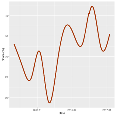
The metric we are going to look is the share of half hourly operational demand met by wind generation from 1 September 2015 to 16 January 2017 (the period of the 2016 blackout has again been excluded). The smoothed trend in the share of operational demand met by wind is shown in Figure 20. The most striking point is the sharp increase in the share of wind in the second quarter of 2016. This is due to several factors including seasonal variation in wind generation, the closure of the Northern coal fired station and additional wind generation capacity being brought on line.
Figure 20 The smoothed trend in the share of operational demand met by wind in South Australia: 1 September 2015 to 16 January 2017
What is more interesting is the reliability wind in meeting this increased proportion of demand, particularly when demand is high, as for example peaks in summer and winter. What would like to see is how the volatility of the share of operational demand met by wind is changing over time, at time scale that matches up with the problem of managing intermittent wind generation. A bit of work needs to be done.
First, the standard deviation of the change in the share of operational demand met by wind is calculated at successively longer time scales; over a half hour, over an hour and so forth. Longer time scales can be created by taking the difference of averages, as for example, the difference in hourly, daily and weekly averages. However, this dampens temporal correlation and variability. Longer time scales can be created by taking successively longer differences in the share of operational demand met by wind without averaging, say from 9:00 to 9:30, 9:00 to 10:00, 9:00 to 11:00 and so forth. This preserves temporal correlation and it is temporal correlation that gives rise to large swings in wind generation and demand. This raw variability, which is still tied to a five-minute interval, is a measure of how much things can change over a given length of time.
The change variability over longer time scales is shown in Figure 21. The variability in the share of operational demand met by wind increases but at a decreasing rate. For instance, there is a sharp increase in variability over the first four hours but this progressively slows and eventually plateaus at 18 hours. After 18 hours, the temporal correlation in the change in share of operational demand met by wind is essential gone. We can use this measure of variability to calibrate a useful picture of how volatility has been changing over time.
Again, a two-stage smooth is used to extract the trend in volatility over time, this time calibrating the smooths to approximate the volatility to a time scale of about two hours. This is done by matching standard deviation of smoothed volatility to about 10 per cent which corresponds to about two hours in Figure 21. The motivation is to try and get a picture of how the scope of problem of managing intermittent generation has changed in South Australia.

Figure 21. The standard deviation in the share of operational demand met by wind generation over successive time periods in South Australia: 1 September 2015 to 16 January 2017
The first stage smooth, which takes into account the expected pattern of diurnal variation, can be interpreted as the mean or expected share at a point in time. The deviations from trend represent volatility or uncertainty about the expected level demand met by wind. This uncertainty is managed through capacity to adjust the output of dispatch from generators at the same time scale as the volatility. The trend in volatility is obtained by taking successively finer smooths of the deviations from trend until their variability matches the variability of the share of operational demand met by wind over two hours (as shown in Figure 21). Over this time span the flexibility to manage variability comes from generators that are online that can adjust output, fast start new generators that can be brought on line and the ability to import and export energy to Victoria.
The result, which is intended to be illustrative, is shown in Figure 22. The dark orange bands show expected diurnal pattern in the share of operational demand met by wind. The pattern within the band is constant over each 24 hour period and is repeated so frequently that it fills the band with a solid colour that has been made translucent. The edges of the band are the upper and lower bounds of the expected diurnal variation. The overall pattern jumps sharply toward the end of the first half of 2016 as was seen in figure 20.
The light orange line is the deviation about the diurnal pattern and is the volatility or the uncertainty that needs to be managed. For the most part, volatility falls within the band of diurnal variation but there are spikes that lie well outside these bounds and they occur quite frequently. These spikes are ramp like events are created, for the most part, by irregular cycles in wind speed that were shown in the previous blog. The time from peak to trough would be the order of four hours. The escalation of uncertainty in the second half of 2016 is quite clear, particularly from late June into September, where the magnitude and the frequency of the peaks and troughs are sharply elevated.
Figure 22 The expected diurnal pattern and the volatility of the share of operational demand met by wind: 1 September 2016 to 16 January 2017

The light orange line is the deviation about the diurnal pattern and is the volatility or the uncertainty that needs to be managed. For the most part, volatility falls within the band of diurnal variation but there are spikes that lie well outside these bounds and they occur quite frequently. These spikes are ramp like events are created, for the most part, by irregular cycles in wind speed that were shown in the previous blog. The time from peak to trough would be the order of four hours. The escalation of uncertainty in the second half of 2016 is quite clear, particularly from late June into September, where the magnitude and the frequency of the peaks and troughs are sharply elevated.
Wind generation in South Australia was a primary driver of the volatility of residual demand over the winter month in 2016. However, the relationship between demand and wind also contributed. Demand and wind generation output were negatively correlated. That is, higher than average demand is associated with lower than average wind generation. Over the entire period this correlation was only about 12 per cent but this jumped to 25 per cent in July and August of 2016.
Meeting demand with a high proportion of wind generation is, as hypothesis at start of this blog suggested, one factor that is likely to be a source of increased price volatility in South Australia. Other factors may be a prerequisite or of equal or greater importance. Infrastructure is brought into the picture in the next blog